By Alex Smithers
Anybody who’s lived in a small town is probably used to receiving directions like, “Oh, I live in the house with the blue roof behind the Coop,” or “The Country Food store is just past the Arctic Survival Store.”
When I moved to Iqaluit from Toronto in October of 2019, not only was it my first time living in a city not built on a grid, but my first time having to navigate without knowing the landmarks or having Google Maps to guide my every turn.
Unlike most places where addresses are based on streets with ascending numbers, in Iqaluit every building is given a unique number. This means an address can be specified with only a number—a convenient shortcut for Iqalummiut, but tricky if you just moved to town and are trying to drop off a résumé somewhere.
To make matters worse, Google Maps doesn’t respond well to a search for just a number. It’s more likely to return a Baskin Robbins touting its variety of flavours than the “building 31” you’re searching for.
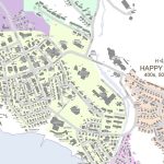
Fortunately, being spotted wandering around aimlessly in the freezing cold, a community member let me know that there’s a better way. The City of Iqaluit published a PDF in 2018 with every building number on it.
Here is a detail of the downtown area:
Can you find the Pinnguaq Makerspace, building 1412?
Even with the help of this PDF, I started thinking, “wouldn’t it be nice if there was an online lookup service that would allow you to input a building number and see its location on a map?”
So I created one.
How I Did It
To build the service, I followed four basic steps:
- Find all the alphanumeric characters on the map
- Identify those characters using machine learning and extract the building numbers (this will be the main focus of this article)
- Figure out the geographical coordinates of the building numbers
- Integrate the number and coordinate data with a mapping service
Step 1: Locating Alphanumeric Characters
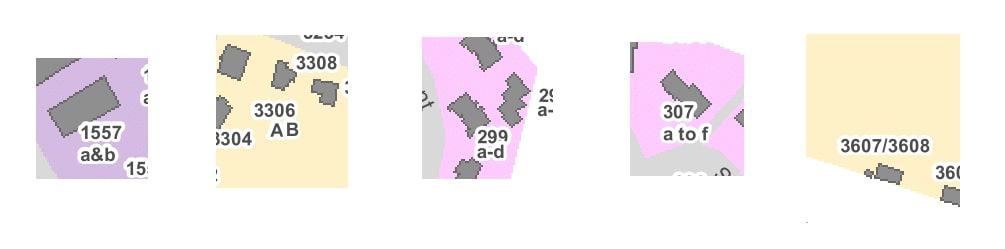
Let’s start by taking a closer look at a section of the map:
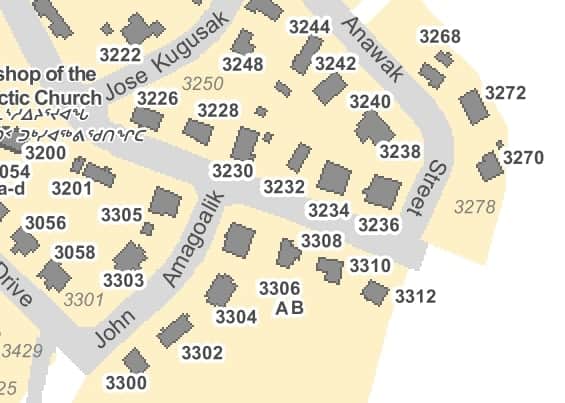
Fortunately, all the numbers have been coloured the same shade of grey, so starting at the top left of the map, we can scan pixels, looking for ones that match that colour. Whenever one is discovered, we then walk through all neighbouring pixels to define bounds for that number.
In the example above, the red arrows indicate scans of numbers that are not the desired shade of grey. Once a grey pixel is found (for example in the top left of the number two), we mark it as found (green) then look to see if any neighbors are grey as well. If they are, we mark those as found, then look into their neighbors. This process is continued until no new grey neighbors are found, at which point we save that number and its location for future processing.
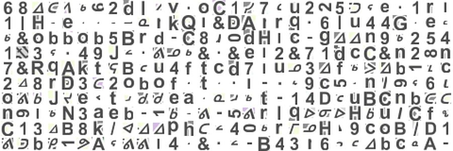
The result of doing this scan across the entire map yields a hodgepodge of numbers and letters:
Step 2: Number Identification
Going through the 6,500 characters found on our PDF is a big task for a human, but a small one for a computer. But how can we get a computer to tell the difference between a “3” and a “9”, let alone similar looking characters like a “B” and an “8”, a “7” and a “T” or a “4” and an “A”?
A first approach might be to define a rough shape of adjacent pixels for each character we want to identify and see if a given input follows that shape. For example, take a black pixel and say “If we can walk right 3 times and then go down and to the left 4 times, we have a seven.”, and do something similar for every character. However this will run into problems: defining a general shape won’t be trivial, processing will be expensive, and numbers can range in position and size, be cut off or have “noise”. This would be a “classical” artificial intelligence approach to solving this problem, where we attempt to design an algorithm that uses a set of logical steps to identify a character.
Fortunately, machine learning offers another approach to artificial intelligence and provides a much more feasible solution to our problem. In order to identify a given character using machine learning, we set up a network of weights—a multiplier that will allow something to express itself more strongly or weakly—that will then take a set of pixels and output how likely it is to match each possible character. This is called a neural network.
Neural Networks
Neural networks are meant to simulate the way that 100 billion neurons in the brain allow us to think. These neurons are made up of a head (soma) with dendrites capable of detecting chemical signals (neurotransmitters) and a long body (axon) with terminal buttons that release signals of their own. A critical mass of neurotransmitters around the soma will trigger a message for the terminals to release, in turn causing neurons down the line to fire in a chain reaction. In this way the neurons in our heads can convert the visual input into recognition that what we’re looking at is a number.
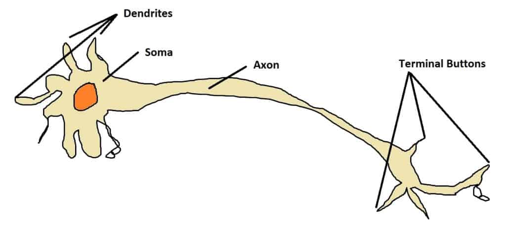
In a neural network we substitute biological neurons for “nodes”, which take multiple inputs and give an output value. Like neurons, nodes can be chained together to perform abstract calculations such as converting a series of pixel values into a single number.
To better our understanding, let’s take an example of a household getting a pet dog.
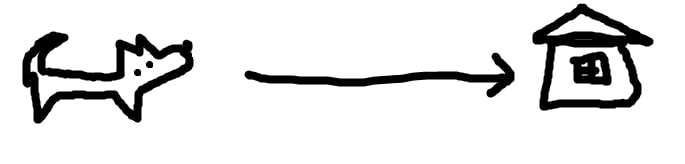
Imagine that we are going to be called by The Humane Society and we have to decide whether or not we are going to adopt a certain dog. We will be told how obedient the dog is on a scale of 0-10, and will process this information using our neuron, adopting it if the output is greater than 5.
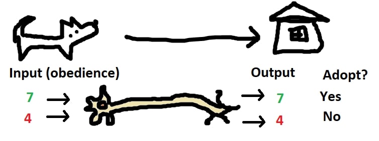
The most simple way we could process the input would be to pass it directly through to the output. But what if we really wanted a dog and would adopt the least obedient dog on earth? We could bias the input by adding a value to the input.
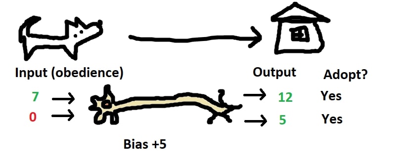
What if we actually want a dog to train, and don’t want a dog that’s obedient to begin with? We could apply a weight to the input by multiplying it against a negative number.
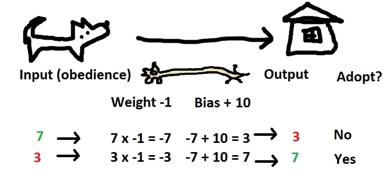
We can also use this method to take into account multiple inputs. If we wanted a very small, somewhat obedient dog, we could use the following weights/values:
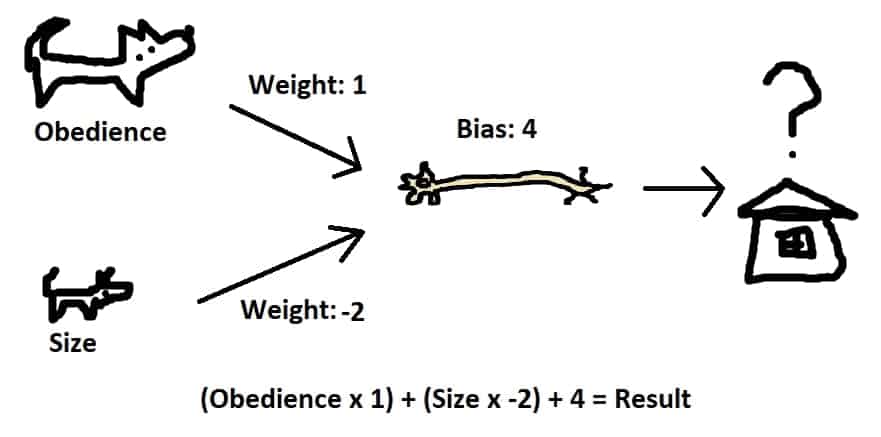
Some sample values in a table yield:
| Size | 10 | 0 | 10 | 0 | 2 | 4 |
| Obedient | 0 | 10 | 10 | 0 | 6 | 8 |
| Result | -16 | 14 | -6 | 4 | 6 | 4 |
Here we can see that when size is low and obedience is high we get a large result. Also we can see that a low size is more important than high obedience. We will add one last piece to the neuron puzzle: an activation function applied to the result of the weight-bias calculation. There are many options here, but we will use the Rectified Linear Activation Function (ReLU) that returns 0 in place of any negative number. This is similar to a biological neuron’s working, where it won’t fire unless a threshold is passed. Applied to the table above would yield:
| Size | 10 | 0 | 10 | 0 | 2 | 4 |
| Obedient | 0 | 10 | 10 | 0 | 6 | 8 |
| Result | -16 | 14 | -6 | 4 | 6 | 4 |
| ReLU | 0 | 14 | 0 | 4 | 6 | 4 |
A few inputs into a neuron will allow for a simple decision to be made, but a network of neurons is required to decide more complicated systems.
Let’s say we’re looking for a dog for our grandmother who is hard of seeing, and have information on how big the dog is and how much it barks. So that grandma can find her dog, we want it to be either big or barky. We don’t want it to be both big and barky though, as while it would be (too?) easy to find, it might scare the neighborhood children.
This system is logically equivalent to an “exclusive or,” requiring either A or B but not both, and no combination of weights and bias can model it. Feel free to give it a try on your own.
By adding what’s called a “hidden layer” of neurons between our inputs and our output neuron, we can create a model of this system:
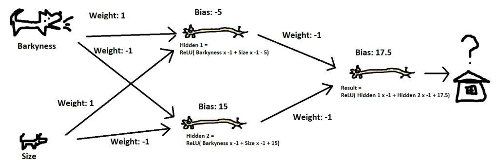
This network computed with some sample values yields what we desire:
| Loud | 0 | 0 | 10 | 10 |
| Big | 0 | 10 | 0 | 10 |
| Hidden 1 | 0 | 5 | 5 | 15 |
| Hidden 2 | 15 | 5 | 5 | 0 |
| Result | 2.5 | 7.5 | 7.5 | 2.5 |
We’ve now seen how a neural network can be used to decide a few levels of problems. Pushing this progression further, more complicated networks might have additional inputs (colour, age, hair length) or multiple outputs (Do we adopt the dog, give it to grandma or decline?). These more complicated networks can be satisfied by increasing the number of hidden layers and nodes, but this also increases the weights and biases that need to be assigned.
Training a Network
In our previous example we used some basic intuition to set up our network, but it’s going to be difficult to intuit thousands of weights across hundreds of nodes when it comes to identifying characters on our map. This is where machine learning comes in, offering a way to programmatically update weights and biases over time and improve the performance of the network.
Let’s take another look at adopting a dog, but assume we don’t have any idea what we’re looking for. We may as well take a guess with our adoption, which would be equivalent to assigning random weights to our network. The network below for a dog with weights “obedience” 3 and “size” 8 gives a score of -13. In the name of science though, let’s adopt it and see how it goes.
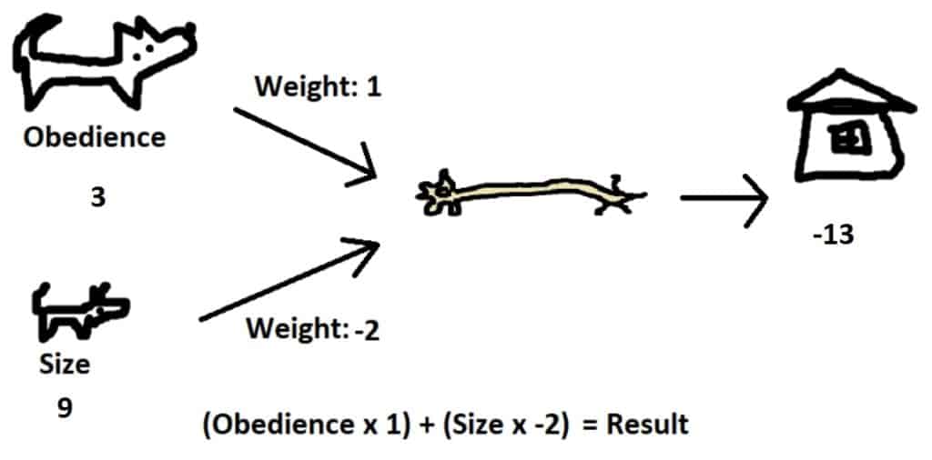
If we find that our dog is actually perfect for us, this means the output of our network should have been 10, not -13. From here we can try to adjust our weights to be more accurate. The “size” weight of -2 multiplied by 8 played a large role in yielding an incorrect value, so should be largely adjusted, whereas the “obedience” weight pushed us in the right direction but did so based on a small value, so it just merits a minor adjustment.
Imagine a few years later we adopt another dog with obedience 9 and size 2. With adjusted weights of obedience: 1.5 and size: 0.5, our network evaluation looks as follows:
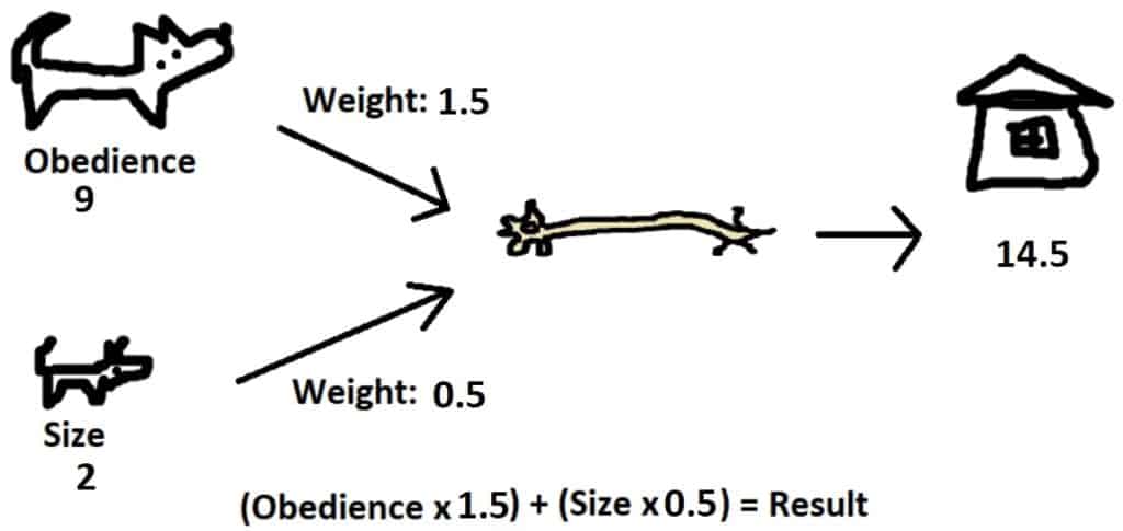
If this dog doesn’t really fit in with our family, it might mean a proper score would be 2 instead of 14.5. We might adjust weights to lower the score, slightly reducing the “size” weight and heavily reducing the “obedience” weight.
Each set of inputs (obedience and size) in combination with an actual result (how the dog fit in) makes up a piece of training data. Over the course of a lifetime, we could adopt a number of dogs, and each time slightly improve the weights on our network until it approaches values where it accurately predicts a dog’s compatibility with our family.
While this example is greatly simplified in comparison to training a multi-layered network with numerous inputs and outputs, the approach of comparing the network’s results to real world results and tuning weights to improve accuracy stands. In practice, the Backpropogation algorithm will calculate weight adjustments to minimize the loss (or difference between results and expected output) of a network. This process is far from fool-proof, requiring careful network setup and very large sets of training data, but can be leveraged to solve problems such as identifying characters from our map.
Data Preparation
In our map, there are 26 different characters that will need to be identified, 0-9, a-f, t, o, A-D, /, &, -, and ‘other’. This will form the 26 possible outputs of our network, where the output assigned the highest value will be it’s guess of the character.
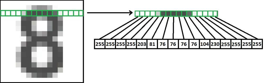
As for the inputs, we will take an image of a character, and resize it into a 16×16 grayscale pixel image. This will create 256 values ranging from 0 to 255 that will serve as the input to the network.
As with adopting dogs to tune our network in the example, we‘ll need training data for character identification. Generating this required manual identification of numbers, looking at a few hundred characters pulled from our map and putting them into corresponding folders. Once created, Google’s Tensorflow did the heavy lifting training the network. After some test runs, two hidden layers of 128 and 64 nodes lead to 98 per cent accuracy on test data.
Knowing that the network isn’t perfect, I set up a manual identification process for any character with less than 70% certainty. Here are some examples:
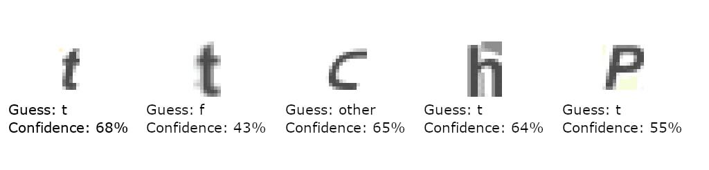
With the characters identified, the final steps were to plot their positions relative to the real world and then put the results in an online database. With mapping service provided by OpenStreetMaps and Mapbox, finding the Iqaluit Makerspace (building 1412) is now just a little bit easier.
